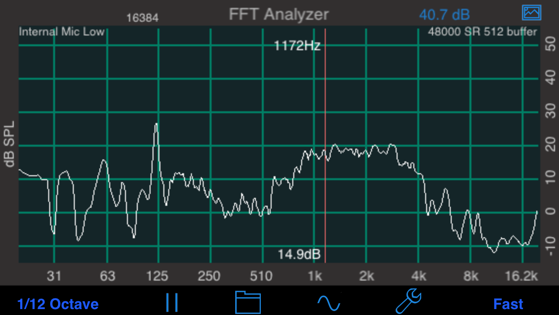
FFT is a high-resolution audio analysis tool available as an in-app purchase in AudioTools. It uses the Fast Fourier Transform (see below) to analyze incoming audio, and displays a very detailed graph of amplitude vs. frequency.
NOTE: This information applies to the FFT module available within AudioTools. The standalone app is older, and does not include every feature mentioned here.
✨ Master your setup: Follow our new Sound System Setup Guide for a quick, pro-quality result.
Don’t know if you should download FFT or RTA? Check out our comparison page for more information.

Available in AudioTools on the App Store
Demo video of FFT.
This application has been designed for acoustics work, and so the FFT bins have been normalized to octaves, to get a display that will show a flat line for pink noise. You can control both the level of graph smoothing and decay time, to get as much or as little detail as you require.
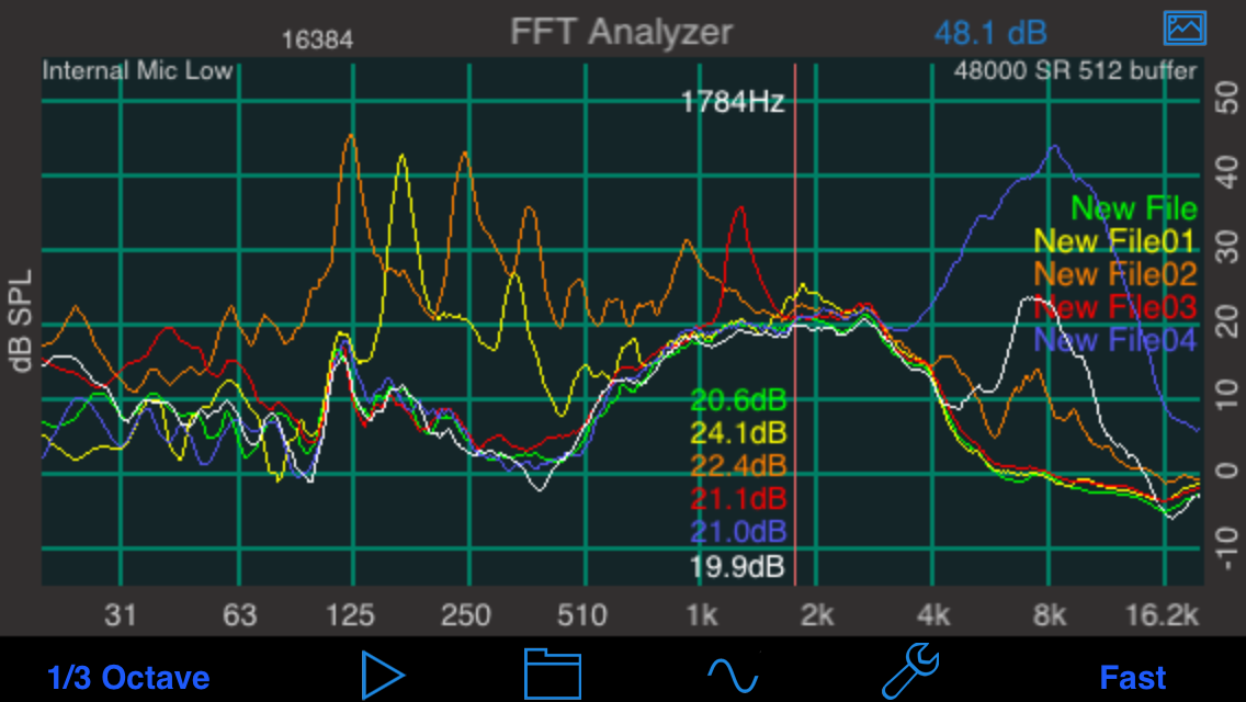
FFT showing multiple recalled measurements, on iPhone.
FFT also includes support for the optional Reference Curves feature.
This example shows using a single reference curve, with a +/- dB range to say whether or not the live curve is within that range. The green dot shows that this curve passes.
See our “dB vs. dB” page to understand what the SPL numbers mean, and why they might be different on different modules.
Features:
- FFT size from 4096 to 32k (on newer iOS devices)
- Difference mode to compare 2 graphs
- Peak frequency readout in real time
- Signal generator can generate sine waves, square waves, white noise, and pink noise.
- Cursor: Move your finger across the screen to get a cursor to read out exact dB levels and frequencies
- Touch-GUI: use pinch gestures to scale the graph and zoom in on frequencies.
- Double-tap to normalize the graph to full range, and fit the entire graph on the screen.
- Both full range (20-20kHz) and low range (5Hz to 3100Hz) are available.
- Overall dB display
- Save the graph image to your photo roll to include in a report
- Export the data in XLS format.
- FFT windowing available
- RPM of cursor position or peak frequency
- Music note of cursor position or peak frequency
See the sections below for more information about running and configuring FFT.
FFT Configuration Examples
Analyze Speaker Response: Use Pink noise as the test signal, select Equal Points Per Octave, select 1/6 or 1/3 octave smoothing, select 1s Decay time.
Music Analysis: Signal generator off, select the 2048-point FFT, 0.5s Decay, 1/24th octave smoothing.
Bluetooth and Airplay Output
See our information about using Bluetooth or Airplay.
Operation
Smoothing
Select Octave, 1/3 octave, 1/6 octave, 1/12 octave, 1/24 octave, or none. Smoothing averages the FFT dB values around each graph point logarithmically.
Decay Mode
The decay times apply to the graph dB values. A decay time of one second will cause a point to decay at the rate of 20dB/second. Peak Hold holds the highest value received, and Average is a true linear average of all readings over the time of the average. To clear Peak or Average mode, select another mode momentarily and then go back to Peak or Average mode.
NOTE: In EPPO mode, the decay time on the lower octaves is the same as the upper octaves, but since they are not being refreshed as often, the will jump up and then decay back down.
Graph Scrolling
The graph will scroll up and down when you slide one finger up and down on the screen.
Use a two-finger vertical pinch to adjust the screen scale, to see more or less dB on the screen. Use a horizontal open-pinch gesture to spread out the screen and zoom in on the frequency axis. When the frequency scale is zoomed, you can use two fingers to pan the graph horizontally.
At any time, double-tap the screen to normalize it. This will show the full frequency range, and fit the graph to the screen.
The state of the graph is stored as you make changes, so the next time that you start the FFT app, the zoom and scale settings are restored.
Cursor
Swiping left and right will bring up a cursor, which you can dismiss by swiping off the graph to the left.
Generator
Touch the sine wave icon to bring up the built-in generator. You can select your signal type, and for sine and square waves, the signal frequency. Note that digitally-produced square waves start to alias badly above about 2000 Hz, so you will get audio artifacts.
The generator frequencies always change smoothly, to prevent zipper noise, and turn on and off with soft muting.
Like the other calculations, the generator waveforms are created digitally using 64-bit floating point math, and are very accurate and low-distortion. Note that we have found that running the headphone output 1 click below maximum yields the lowest distortion waveforms.
File Save and Recall
Tap the folder button to access the AudioTools advanced and complete save/recall system. See the Save / Recall page for full details.
Overall dB Display
The overall, unweighted SPL level is shown at all times on the screen in the upper right-hand corner. This is the same value that is shown on the calibration screen.
Clipping
If clipping of the input occurs, the words “Clipping Detected” will be displayed above the graph in the upper left-hand corner in red for 1.5 seconds.
Save to Photo Roll
Tap the picture frame button in the upper right corner to store the actual graphical image from the main screen to the device’s photo roll, minus the control settings. If you want the complete image, just use the normal iOS screen capture function.
Saving Multiple Averaged FFT Plots
You can create a single plot that is the average of a number of previously stored plots by turning on Average Plots on the Setup page, and then recalling all of the saved plots. The main screen will show something like “5 Graphs”. Now, before saving this average, go back to the Setup page, tap the microphone icon at the top, and select the choice for “Disable Audio Input”. Now, when you save the plot using the normal Save/Recall page, the average will be stored.
In the same manner, you can save other sets of stored plots into a new file. Then, to compare them, go to the Save/Recall page, and on the mini-menu, select “Clear Recalled Graphs”. Turn off Average Plots on the Setup page, and now you can recall the averaged files that you just saved, and they will appear as individual plots.
Setup
Full Range / Low Frequency Mode
Full Range shows 20-20kHz range, while Low Frequency mode shows 5Hz to 3100Hz.
Audio Pass-Through
Turn on or off to allow audio that is coming in to the unit to be presented at the output. Turning on the generator overrides audio-pass through.
Difference Mode
This switch turns difference mode on and off. When turned on, the most recently recalled graph (if any) is used as a baseline for the FFT function. In other words, the recalled graph is subtracted from the current FFT graph.
You can use Difference Mode to compare speakers, or do a before and after comparison of an acoustic space.
FFT Size
Choose the size of your FFT on the setup screen. The larger the size of the FFT, the more resolution you will have, but the slower the response time. If you choose Equal Points Per Octave, each octave will have high resolution (equivalent to the upper half of a 512 point FFT), but the lower octaves will update much more slowly. Use this mode for steady-state sound inputs, such as pink noise. (See the section above for more information about FFT size).
FFT Windowing
When turned on, the data is windowed before sending it to the FFT. This has the effect of reducing noise artifacts, and allowing greater dynamic range on the FFT. With windowing turned on, you can get greater than 100dB of dynamic range when looking at sine wave signals.
Peak Tracking
Turns peak tracking on, showing the frequency either on the cursor, or in large text on the screen. Our algorithm uses the actual highest FFT bin, and does not use the calibration compensation, so it may not be the highest point on the graph.
Input Source
This is the standard AudioTools input source selection screen, where you can choose microphone gain, or change settings.
About the FFT Calculation
FFT stands for Fast Fourier Transform, which is a mathematical algorithm that breaks a signal into frequency bins. Each bin is the same size, in Hertz. The size of the FFT determines the width of the bins in Hertz. Bin width = sample rate / FFT size. Since we are running at the iPhone’s maximum sample rate of 48000 samples/second, for a 1024 point FFT each frequency bin would be 48 Hz wide. This is gives us great resolution at 10kHz, but poor resolution at 32 Hz.
We can run larger and larger FFTs, but since we first have to store up all the samples to fill the FFT, and then do the math, the lag time starts to increase and the display becomes less and less responsive.
In FFT, we provide the choice of FFT size, currently from 4096 points to 16,384 points (32,576 on the newer iOS models). In addition, we provide another mode, which we call Equal Points Per Octave (EPPO). In this mode, we run a fairly small FFT (currently 512 points), but we only use the top octave from this FFT. So, we get a resolution at 10kHz of about 93Hz. Another way to look at it is that we get about 120 data points in the top octave (think of it as 1/120th octave resolution, which is about right). Then, we decimate and filter to get the sample rate down to 24kHz, and then run another 512 point FFT. So again, we get 1/120th octave resolution. We continue this process right down to the lowest octave. The result is excellent resolution across the frequency spectrum. The cost is that each octave only updates half as quickly as the octave above it, so the low octaves update much more slowly. The upper octaves retain very quick response.
EPPO is best used with steady-state signals, such as pink noise, or to analyze constant noise signals. If you want to see the entire graph updating quickly, use 4096 or 8192 points. Note that due to the fact that there are individual FFTs running for each octave, you may see graphical anomalies in the noise floor — for example, since the decimation filter cuts off frequencies above the Nyquist frequency, the lower FFTs don’t even get the higher frequencies, and so might have a lower noise floor than the upper FFTs. This is normal. You can adjust the graph to move the entire FFT noise floor off the bottom of the screen to get a cleaner looking graph.
All calculations are done in 64-bit floating point for the best accuracy and to get the lowest possible noise floor